OceanParcels

OceanParcels, “Probably A Really Computationally Efficient Lagrangian Simulator”, is a set of python classes and methods that is used to track particles like water, plankton and plastics. It uses the output of ocean general circulation model (OGCMs). OceanParcels main goal is to process the increasingly large amounts of data that is governed by OGCM's. The flow dynamics are simulated using Lagrangian modelling (observer moves with particle) and the geophysical fluid dynamics are simulated with Eulerian modelling (observer remains stationary) or provided through experimental data. OceanParcels is dependent on two principles, namely the ability to read external data sets from different formats and customizable kernels to define particle dynamics.

Concept

OceanParcels takes a flow field given through Eulerian methods or experimental data (e.g. provided through land-based measurements, satellite imagery or Doppler currents) as input. This data can be given on various grid structures. To obtain data at an arbitrary point, interpolation is used. Lagrangian modelling uses the data given by the flow field and interpolation to simulate the dynamics of an object.

Grid structure

Figure 1: Grid structures in horizontal and vertical direction.

Figure 2: A grid (left), B grid (middle), C grid (right)

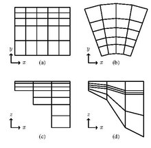
In the horizontal plane, i.e. in the x-y-plane, OceanParcels allows for rectilinear and curvilinear data grids (see Fig. 1 a and b respectively). In the vertical plane, i.e. the x-z-plane, z-levels and s-levels are supported (see Fig. 1 c and d respectively). All four combinations of these grids are supported in three-dimensional space.

OceanParcels also supports so-called staggered A, B and C grids, which are common in ocean modelling. These take into account that the different variables can be measured at different grid points. The relevant variables in Ocean analysis are the meriodial velocity (v), the zonal velocity (u) and the Tracers (q). In an A grid all of these are evaluated at the same grid points. In a B grid, u and v are evaluated at the grid point in the center between the grid point where T is being evaluated, that is there are two overlying grids. In a C grid all variables are evaluated on their own grid, that is there are three overlying grids. See Figure 2 for a visualization.

Interpolation methods

To obtain field data at a point that is not on a grid node, interpolation methods are used. OceanParcels supports several different such methods:

• linear interpolation
• nearest-neighbor interpolation
• interpolation on A, B, C grids.

Lagrangian modelling

The Lagrangian trajectory of a particle can be calculated by numerically integrating over its position $X$ as a function of time, given by $X(t_{2})=X(t_{1})+\int _{t_{1}}^{t_{2}}v(x,\tau )d\tau +\Delta X_{b}(t_{1})$. Here $t_{1}$ is the starting time and $t_{2}$ is the time at which the position of the particle is evaluated. $v(x,\tau )$ is the velocity of the particle at time $\tau$. $\Delta X_{b}(t)$ captures the movement of the particle caused by its specific characteristics (e.g. an ice-berg moves differently in the ocean than a non-frozen water mass). Unless otherwise specified, OceanParcels uses a fourth-order Runge-Kutta scheme for the integration of this function. As alternatives, OceanParcels supports Euler-forward integration or adaptive Runge-Kutta-Fehlberg integration.

OceanParcels provides the option to model individual behavior of a particle. Individual behavior is behavior that is defined by characteristics of a particle, for example icebergs melt and fish swims, leading to different dynamics. OceanParcels implements this using short pieces of code that are executed whenever a ParticleSet (class defining the particles used) is executed. Those pieces of code are called kernels. Some commonly used kernels are predefined in OceanParcels, such as kernels modeling Brownian motion. However, the user may also define problem specific kernels. This allows for modeling various objects, examples of which are given in the section "Applications". For implementing these customized kernels the user can choose between using Python with a possibility to automatically translate to C or using a C-library.

Applications

Lagrangian analysis can be used to simulate the pathways of virtual particles, which can represent water masses, temperature tracers, salinity tracers, nutrient tracers, kelp, coral larvae, plastics, fish, icebergs, plankton, etc. The pathways of the different particles can be modelled using specific kernels, for example that fish can swim and that icebergs can melt.

Water masses

The movement of water masses can be calculated numerically using velocity fields, which are simulated by a primitive equation model (fine resolution Antarctic model). Using this model, it can be estimated how many times the water mass has traveled around Antarctica and how much time it has spend in the Southern Ocean. It turned out that on average a water mass travels around Antarctica six times before it is reaches the surface for the first time.

Temperature tracers

Surface temperatures can be analyzed using proxies, which can reconstruct environmental changes over the last 600 years. These reconstructions are based on alkenones, Membrane lipids and stable isotope ratios of globigerinoides ruber. It is argued that ocean currents are transporting these proxies far away from there origin, creating a bias towards temperature approximations.

Salinity tracers

The proxies used for salinity are the ratios between elements and calcium and stable oxygen isotopes ratios of foraminifera. These isotope ratios can be calculated by the following formula: $\delta ^{X}={\frac {^{x/y}R_{sample}}{^{x/y}R_{reference}}}-1$, where y is the common isotope and x the more rare isotope. Both ratios have a positive correlation in the Mediterranean Sea, which has a strong west to east salinity gradient. Salinity tracers are important for reconstructing the ocean circulation, because together with temperature, the density can be determined, which can reconstruct large-scale circulation patterns, including meridional overturning circulation.

Nutrient tracers

The influence of the Equatorial Undercurrent (EUC), New Guinea Coastal Undercurrent (NGCU) and the New Ireland Coastal Undercurrent were examined using models to elucidate the high iron concentrations in the Pacific Ocean. During El Niño, the latter two currents strengthen, which enhances the iron concentrations in the Pacific.

Plastic

Lagrangian particle models have shown that about three quarters of buoyant marine plastics released from land are ending up in coastal waters, with the highest concentration in Southeast Asia. However, these simulations are overestimated with respect to field measurements.

Fish

The transport of fish larvae by ocean currents is an important dispersal mechanism, because the timing has a lot of influence on the location where the larvae are settled. Pomatomus saltatrix is a fish species that is present globally, and its dispersal is examined by using particle tracking simulations. Especially the East Australian Current is important for maximum dispersal of the larvae.

Plankton

Plankton are important archives to reconstruct past conditions of the ocean surfaces. While the plankton sinks to the sediments, it can be advected by turbulent ocean currents. Ocean simulations can be used to define ocean bottom provinces based on the particle surface origin locations.

Icebergs

The influence of icebergs on sea ice can be modeled and compared to observations. When icebergs melt, a large fresh water flux takes place. Around Antarctica, a negative fresh water flux takes place due to sea ice freezing.

Development

The latest version of OceanParcels can be accessed via GitHub. It is constantly being improved, updated and expanded. The code design ensures that this can be done without effecting the user interface. Below you see a list of some possible improvements:

• Implementing support for using Arakawa D and E grids in the interpolation
• Implementing more advanced interpolation methods
• Implementing support for using unstructured grids in the interpolation process
• Implementing new more efficient programming methods
• Implementing further numerical integration methods for the Lagrangian modelling

Alternatives to OceanParcels

The following list contains some code packages with (partially) similar functions as OceanParcels.

• OpenDrift: Project from the Norwegian Meteorological Institute aiming at developing open-source python packages for calculating drift in the ocean and atmosphere.
• TRACMASS: Fortran 90 code calculating particle trajectory using Lagrangian Ocean Analysis.
• Octopus: Fortran code calculating Lagrangian particle directories in the ocean on a C grid.
• Connectivity-Modeling-System (CMS): Open-source fortran code calculating particle trajectories in the ocean, developed by the University of Miami's Rosenstiel School of Marine, Atmospheric, and Earth Science.