von Kármán–Gabrielli diagram

A Gabrielli–von Karman diagram from.

A Gabrielli–von Karman diagram with the y-axis being the lift-to-drag ratio, which is the inverse of specific resistance.

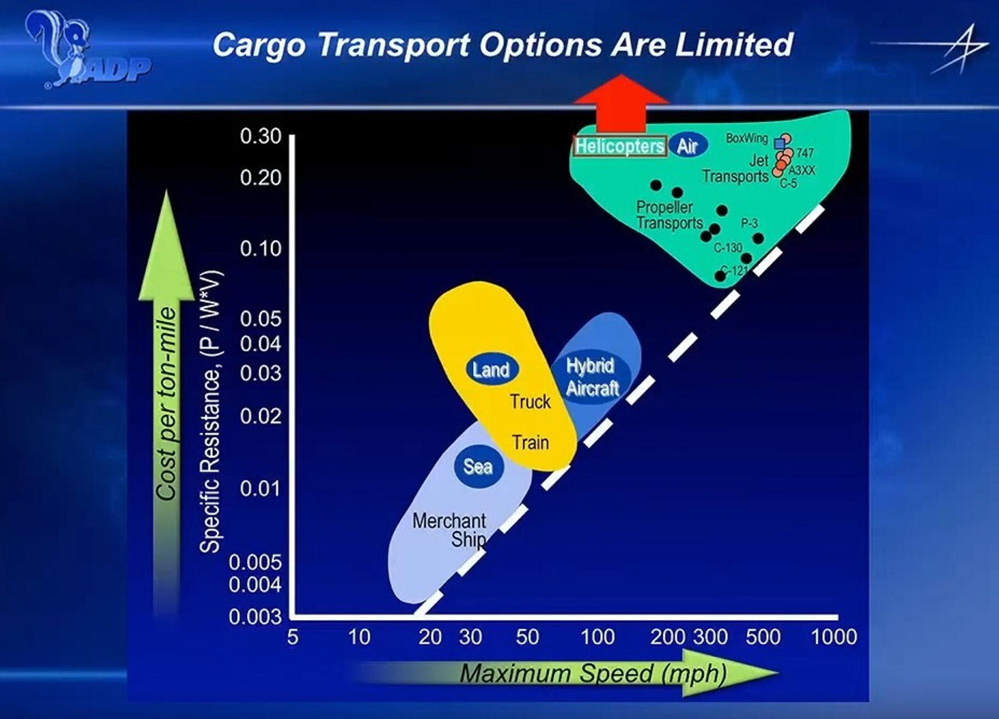
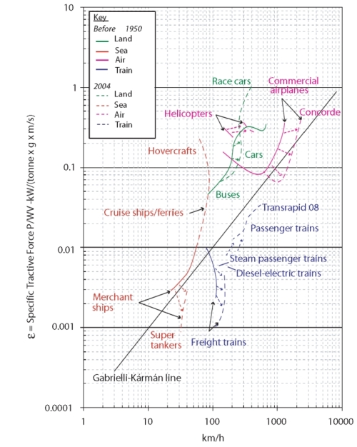
The von Kármán–Gabrielli diagram (also Gabrielli–von Kármán diagram, GvK diagram) is a diagram which compares the efficiency of transportation methods by plotting specific tractive force, or specific resistance (ε = P/mgv = E/mgL) against velocity (v). It was first used by Theodore von Kármán and Giuseppe Gabrielli in their 1950 paper on this subject.

Details

In GvK diagram, the x-axis is the vehicle velocity, and the y-axis is the dimensionless specific resistance. The same kind of vehicle may have multiple different operating velocities, with different corresponding specific resistances, consequently each kind of vehicle generally correspond to a whole region on the GvK diagram, but only the lower-edge of the region is plotted, since specific resistance can always be artificially increased by wasting energy, but not decreased beyond a lower limit depending on the physical and engineering constraints.

The specific resistance is a dimensionless quantity defined by

$$\epsilon :=P/mgv$$

where $P$ is the total power consumption by the vehicle, $m$ is the total mass of the vehicle, $g$ is the gravitational constant, and $v$ is the velocity of the vehicle. The inverse of specific resistance is defined as transport efficiency.

Alternative forms of specific resistance

For example, if we have a freight vehicle in which most of the total mass is in its freight, and we have freight to carry over a distance of $L$, but we have no requirement for how long it should take, then the total energy consumption of the vehicle over the journey is

$$E=Pt=P(L/v)=\epsilon (mgL)$$

so we can interpret the specific resistance as a ratio for how much resistance the vehicle faces. A low resistance means it needs to consume less energy to carry the same load through the same distance.

The power is equal to the drag force times velocity. For aircraft in cruise flight the lift is equal to the weight (L=mg) and the engine thrust is equal to the drag (T=D). Hence,

$$\epsilon =P/(mgv)=D/L=1/f$$

, with f=L/D the lift-to-drag ratio, so the specific resistance of airplanes is roughly equal to the inverse of the lift-to-drag ratio.

The limit line

The original paper by Gabrielli and von Kármán already noted that for all single vehicles they studied, there is a limit of the form $\epsilon \geq Av$, for some constant $A\approx 0.00175\;\mathrm {mph} ^{-1}=4\times {}10^{-4}\mathrm {s/m}$, which exhibits itself as a straight line on Figure 3. The constant $A$ can be interpreted as a measure of inefficiency. For vehicles in a convoy, such as a long train or a group of cars moving in a long tandem, the constant can be improved, decreasing energy dissipation to air resistance. Figure 5 shows a 4-fold improvement.

Technological improvements over the years can move the limit line downwards. For example in 1980, the ultra large crude carrier (ULCC) could reach a limit of $3.6\times {}10^{-4}\mathrm {s/m}$. A report in 2004 demonstrated further improvements.

For vehicles moving through fluid (ships, submarines, planes, etc), the specific energy is a dimensionless quantity defined as the Froude number divided by the specific resistance: $\epsilon _{E}=\mathrm {Fr} /\epsilon$. A 1980 report showed that the specific energy has an upper limit of 200 over all kinds of vehicles moving through fluid, except rocket-powered vehicles (missiles, space rockets, etc) which can reach over 3000 specific energy.

The triangular gap

If land vehicles are excluded from the GvK diagram, then a large triangular "gap" appears, spanned by merchant ship, destroyer, and commercial airplane, with airship being the lone inhabitant of the gap. After the GvK diagram became more widely known to marine engineers, a large number of designs were promoted to fill the gap, such as planing boats, hydrofoils, hovercraft and ground-effect vehicles, without success.

Numerical examples

According to calculations done by Qian Xuesen, a rocket with an average speed of 2 km/s over a 5000 km range would require a thrust of 845,000 N for 140 seconds, with initial mass 44,000 kg and final mass 8,600 kg. This corresponds to $\epsilon \approx 0.2,A\approx 1.0\times {}10^{-4}\mathrm {s/m}$.

1 kWh/100 km has the dimensional units of a force, a resistance force amounting to 36 N.

See also

• Ragone plot

External links

• Diagram for cargo
• Diagram of changes from 1950 to 2004